Analog Methods
Setup
First, let’s import the necessary libraries.
import matplotlib.pyplot as plt
import numpy as np
import xarray as xr

from skdownscale.pointwise_models import AnalogRegression, PureAnalog

# Set style for better-looking plots
plt.style.use('seaborn-v0_8-darkgrid')
Step 1: Load Climate Data
We’ll use the same test dataset as in the BCSD tutorial. This includes:
Training data: Coarse-resolution climate model output
Target data: High-resolution observations
# Define the training period
training_time_slice = slice('1980', '2001')

# Load data from cloud storage
data = xr.open_datatree(
    's3://carbonplan/share/scikit-downscale/test-data.zarr',
    engine='zarr',
    chunks={},
    storage_options={'anon': True, 'endpoint_url': 'https://rice1.osn.mghpcc.org'},
)

# Extract training and target datasets
training = data['training'].to_dataset().sel(time=training_time_slice)
targets = data['targets'].to_dataset().sel(time=training_time_slice)

print('Training data:')
display(training)
print('\nTarget data:')
display(targets)
Training data:
<xarray.Dataset> Size: 2MB
Dimensions:      (point: 5, time: 8036)
Coordinates:
  * time         (time) datetime64[ns] 64kB 1980-01-01T11:30:00 ... 2001-12-3...
    lat          (point) float32 20B dask.array<chunksize=(5,), meta=np.ndarray>
    lon          (point) float32 20B dask.array<chunksize=(5,), meta=np.ndarray>
Dimensions without coordinates: point
Data variables: (12/15)
    DIV          (point, time) float32 161kB dask.array<chunksize=(3, 8036), meta=np.ndarray>
    PREC_ACC_C   (point, time) float32 161kB dask.array<chunksize=(3, 8036), meta=np.ndarray>
    PREC_ACC_NC  (point, time) float32 161kB dask.array<chunksize=(3, 8036), meta=np.ndarray>
    PREC_TOT     (point, time) float32 161kB dask.array<chunksize=(3, 8036), meta=np.ndarray>
    PSFC         (point, time) float32 161kB dask.array<chunksize=(3, 8036), meta=np.ndarray>
    QVAPOR       (point, time) float32 161kB dask.array<chunksize=(3, 8036), meta=np.ndarray>
    ...           ...
    T2min        (point, time) float32 161kB dask.array<chunksize=(3, 8036), meta=np.ndarray>
    T_MEAN       (point, time) float32 161kB dask.array<chunksize=(3, 8036), meta=np.ndarray>
    T_RANGE      (point, time) float32 161kB dask.array<chunksize=(3, 8036), meta=np.ndarray>
    U            (point, time) float32 161kB dask.array<chunksize=(3, 8036), meta=np.ndarray>
    V            (point, time) float32 161kB dask.array<chunksize=(3, 8036), meta=np.ndarray>
    W            (point, time) float32 161kB dask.array<chunksize=(3, 8036), meta=np.ndarray>
Attributes:
    NCO:                        "4.5.5"
    history:                    Wed Mar  1 13:48:35 2017: ncatted -a calendar...
    history_of_appended_files:  Wed Feb  8 14:15:52 2017: Appended file wrf_d...
nco_openmp_thread_number: 1Target data:
<xarray.Dataset> Size: 707kB
Dimensions:  (time: 8036, point: 5)
Coordinates:
  * time     (time) datetime64[ns] 64kB 1980-01-01 1980-01-02 ... 2001-12-31
    lat      (point) float64 40B dask.array<chunksize=(5,), meta=np.ndarray>
    lon      (point) float64 40B dask.array<chunksize=(5,), meta=np.ndarray>
Dimensions without coordinates: point
Data variables:
    Prec     (time, point) float32 161kB dask.array<chunksize=(731, 5), meta=np.ndarray>
    Tmax     (time, point) float32 161kB dask.array<chunksize=(731, 5), meta=np.ndarray>
    Tmin     (time, point) float32 161kB dask.array<chunksize=(731, 5), meta=np.ndarray>
    wind     (time, point) float32 161kB dask.array<chunksize=(731, 5), meta=np.ndarray>
Attributes:
    CDI:                       Climate Data Interface version 1.6.4 (http://c...
    CDO:                       Climate Data Operators version 1.6.4 (http://c...
    Conventions:               CF-1.4
    NCO:                       4.4.5
    history:                   Fri Oct 10 17:54:37 2014: cdo ifthenelse /Volu...
nco_openmp_thread_number: 1Step 2: Prepare Data for a Single Location
We’ll extract temperature and precipitation data for a single point and convert units appropriately.
# Extract temperature data (convert Kelvin to Celsius)
X_temp = training.isel(point=0).to_dataframe()[['T2max']] - 273.15
y_temp = targets.isel(point=0).to_dataframe()[['Tmax']]

# Extract precipitation data (convert to mm/day)
X_pcp = training.isel(point=0).to_dataframe()[['PREC_TOT']] * 24
y_pcp = targets.isel(point=0).to_dataframe()[['Prec']]

print('Training temperature (first 5 days):')
display(X_temp.head())
print('\nTarget temperature (first 5 days):')
display(y_temp.head())
Training temperature (first 5 days):
| T2max | |
|---|---|
| time | |
| 1980-01-01 11:30:00 | 7.229950 |
| 1980-01-02 11:30:00 | 6.005737 |
| 1980-01-03 11:30:00 | 4.625702 |
| 1980-01-04 11:30:00 | 3.686951 |
| 1980-01-05 11:30:00 | 1.733826 |
Target temperature (first 5 days):
| Tmax | |
|---|---|
| time | |
| 1980-01-01 | 7.24 |
| 1980-01-02 | 7.16 |
| 1980-01-03 | 6.53 |
| 1980-01-04 | 4.46 |
| 1980-01-05 | 1.78 |
Step 3: Understanding Analog Selection Strategies
The PureAnalog class supports four different strategies for selecting and using analog days:
1. Best Analog
Selects the single closest analog day
Fastest and simplest approach
Can be deterministic (always same result)
2. Sample Analogs
Randomly samples from the N best analogs
Adds stochasticity to the predictions
Good for ensemble generation
3. Weight Analogs
Uses a weighted average of N analogs
Weights based on similarity (closer analogs get more weight)
Smooths out predictions
4. Mean Analogs
Simple average of N best analogs
Equal weight to all selected analogs
Balances simplicity and robustness
Let’s compare these strategies on temperature data.
Step 4: Apply Different Analog Strategies
We’ll split our data into training and testing periods, then compare the four analog strategies.
# Split data: first 1000 days for training, rest for testing
train_size = 1000
X_train, X_test = X_temp[:train_size], X_temp[train_size:]
y_train, y_test = y_temp[:train_size], y_temp[train_size:]

print(f'Training period: {X_train.index[0]} to {X_train.index[-1]}')
print(f'Testing period: {X_test.index[0]} to {X_test.index[-1]}')
print(f'\nTraining samples: {len(X_train)}')
print(f'Testing samples: {len(X_test)}')
Training period: 1980-01-01 11:30:00 to 1982-09-26 11:30:00
Testing period: 1982-09-27 11:30:00 to 2001-12-31 11:31:00

Training samples: 1000
Testing samples: 7036
# Dictionary to store results (clear any previous results)
results = {}

# Test each analog strategy
strategies = ['best_analog', 'sample_analogs', 'weight_analogs', 'mean_analogs']
n_analogs = 10  # Number of analogs to consider

for strategy in strategies:
    print(f'\nFitting {strategy}...')

    # Initialize and fit the model
    model = PureAnalog(kind=strategy, n_analogs=n_analogs)
    model.fit(X_train, y_train)

    # Generate predictions (extract only the 'pred' column)
    predictions_full = model.predict(X_test)
    predictions = predictions_full[['pred']]  # Keep only prediction column
    results[strategy] = predictions

    # Calculate simple performance metric (RMSE)
    rmse = np.sqrt(np.mean((predictions.values - y_test.values) ** 2))
    print(f'  RMSE: {rmse:.3f}°C')

print('\nAll strategies fitted successfully!')
Fitting best_analog...
  RMSE: 3.065°C

Fitting sample_analogs...
  RMSE: 3.075°C

Fitting weight_analogs...
  RMSE: 2.481°C

Fitting mean_analogs...
  RMSE: 2.322°C

All strategies fitted successfully!
/home/docs/checkouts/readthedocs.org/user_builds/scikit-downscale/envs/latest/lib/python3.13/site-packages/sklearn/utils/validation.py:1406: DataConversionWarning: A column-vector y was passed when a 1d array was expected. Please change the shape of y to (n_samples, ), for example using ravel().
  y = column_or_1d(y, warn=True)
Step 5: Visualize Results
Let’s compare the predictions from different strategies by plotting a 300-day sample.
# Plot predictions for the first 300 days of test period
plot_days = 300
fig, ax = plt.subplots(figsize=(14, 6))
# Plot each strategy
for strategy, predictions in results.items():
ax.plot(
predictions.index[:plot_days],
predictions.values[:plot_days],
label=strategy.replace('_', ' ').title(),
alpha=0.7,
linewidth=1.5,
)
# Plot observations
ax.plot(
y_test.index[:plot_days],
y_test.values[:plot_days],
label='Observed',
color='black',
linewidth=2,
alpha=0.5,
)
ax.set_xlabel('Date')
ax.set_ylabel('Temperature (°C)')
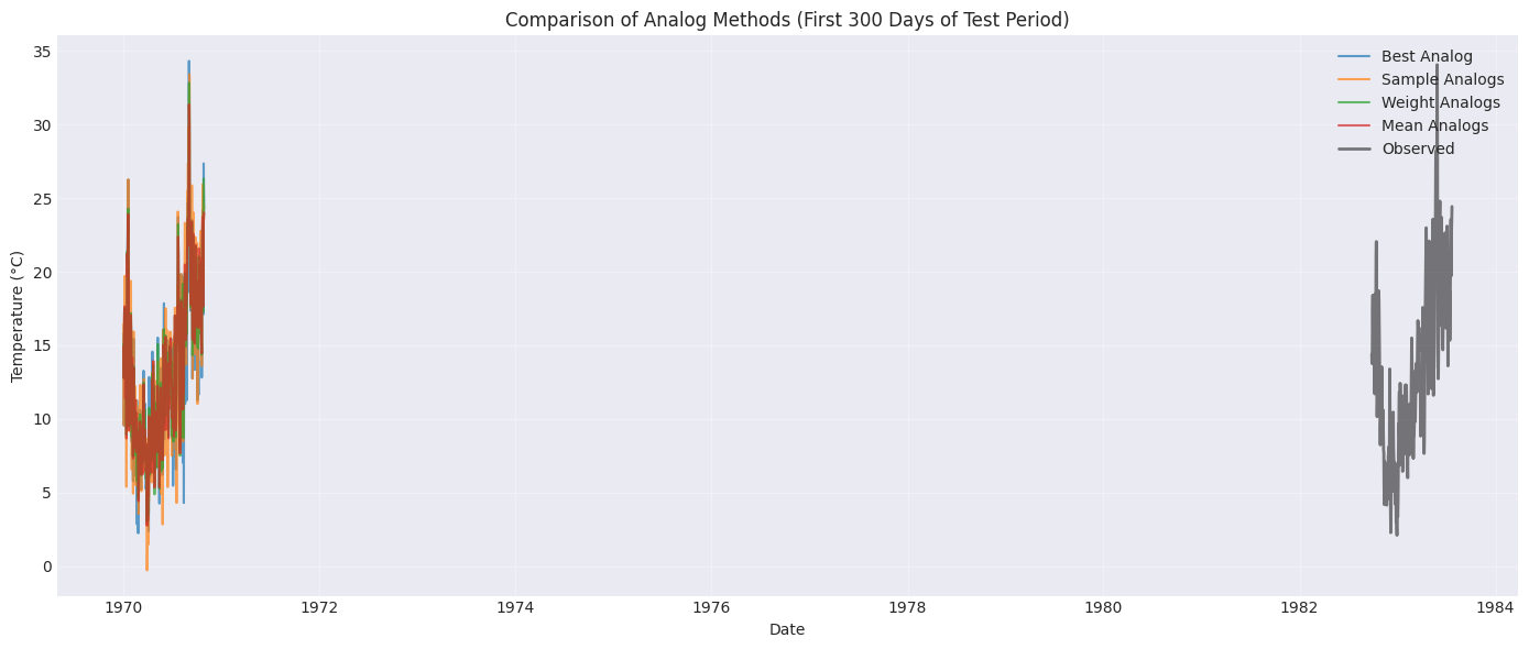
ax.set_title('Comparison of Analog Methods (First 300 Days of Test Period)')
ax.legend(loc='upper right')
ax.grid(True, alpha=0.3)
plt.tight_layout()
plt.show()
Observations
From the plot, you’ll notice:
Best Analog: Can be quite variable, following individual historical days
Sample Analogs: Similar to best analog but with randomness
Weight Analogs: Smoother predictions due to weighted averaging
Mean Analogs: Also smooth, using equal weights
The averaging approaches (weight and mean) tend to be more stable but may miss some variability.
Step 6: Analog Regression
AnalogRegression combines the analog method with linear regression:
Find N analog days
Fit a linear regression using those analog days
Apply the regression to make predictions
This hybrid approach can capture both the analog similarity and systematic relationships.
# Initialize and fit AnalogRegression
n_analogs_reg = 100  # Use more analogs for regression

print(f'Fitting AnalogRegression with {n_analogs_reg} analogs...')
analog_reg = AnalogRegression(n_analogs=n_analogs_reg)
analog_reg.fit(X_train, y_train)

# Generate predictions (extract only the 'pred' column)
predictions_reg_full = analog_reg.predict(X_test)
predictions_reg = predictions_reg_full[['pred']]  # Keep only prediction column

# Calculate RMSE
rmse_reg = np.sqrt(np.mean((predictions_reg.values - y_test.values) ** 2))
print(f'AnalogRegression RMSE: {rmse_reg:.3f}°C')
Fitting AnalogRegression with 100 analogs...
/home/docs/checkouts/readthedocs.org/user_builds/scikit-downscale/envs/latest/lib/python3.13/site-packages/sklearn/utils/validation.py:1406: DataConversionWarning: A column-vector y was passed when a 1d array was expected. Please change the shape of y to (n_samples, ), for example using ravel().
  y = column_or_1d(y, warn=True)
AnalogRegression RMSE: 2.247°C
Step 7: Compare All Methods
Let’s create a comprehensive comparison including AnalogRegression.
# Plot all methods including AnalogRegression
fig, ax = plt.subplots(figsize=(14, 6))
# Plot PureAnalog strategies
for strategy, predictions in results.items():
ax.plot(
predictions.index[:plot_days],
predictions.values[:plot_days],
label=f'PureAnalog: {strategy.replace("_", " ").title()}',
alpha=0.6,
linewidth=1.2,
)
# Plot AnalogRegression
ax.plot(
predictions_reg.index[:plot_days],
predictions_reg.values[:plot_days],
label='AnalogRegression',
linewidth=2,
alpha=0.8,
linestyle='--',
)
# Plot observations
ax.plot(
y_test.index[:plot_days],
y_test.values[:plot_days],
label='Observed',
color='black',
linewidth=2.5,
alpha=0.5,
)
ax.set_xlabel('Date')
ax.set_ylabel('Temperature (°C)')
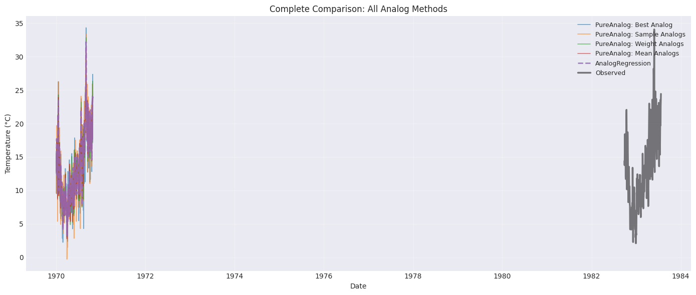
ax.set_title('Complete Comparison: All Analog Methods')
ax.legend(loc='upper right', fontsize=9)
ax.grid(True, alpha=0.3)
plt.tight_layout()
plt.show()
Step 8: Quantitative Performance Comparison
Let’s calculate multiple performance metrics to better understand each method.
import pandas as pd


def calculate_metrics(predictions, observations):
    """Calculate RMSE, MAE, and correlation coefficient."""
    pred_vals = predictions.values.flatten()
    obs_vals = observations.values.flatten()

    rmse = np.sqrt(np.mean((pred_vals - obs_vals) ** 2))
    mae = np.mean(np.abs(pred_vals - obs_vals))
    corr = np.corrcoef(pred_vals, obs_vals)[0, 1]

    return {'RMSE': rmse, 'MAE': mae, 'Correlation': corr}


# Calculate metrics for all methods
metrics_data = []

for strategy, predictions in results.items():
    metrics = calculate_metrics(predictions, y_test)
    metrics['Method'] = f'PureAnalog ({strategy})'
    metrics_data.append(metrics)

# Add AnalogRegression metrics
metrics_reg = calculate_metrics(predictions_reg, y_test)
metrics_reg['Method'] = 'AnalogRegression'
metrics_data.append(metrics_reg)

# Create comparison table
metrics_df = pd.DataFrame(metrics_data)
metrics_df = metrics_df[['Method', 'RMSE', 'MAE', 'Correlation']]
metrics_df = metrics_df.round(3)

print('\nPerformance Comparison:')
print('=' * 60)
display(metrics_df)
Performance Comparison:
============================================================
| Method | RMSE | MAE | Correlation | |
|---|---|---|---|---|
| 0 | PureAnalog (best_analog) | 3.065 | 2.357 | 0.907 |
| 1 | PureAnalog (sample_analogs) | 3.075 | 2.358 | 0.906 |
| 2 | PureAnalog (weight_analogs) | 2.481 | 1.883 | 0.938 |
| 3 | PureAnalog (mean_analogs) | 2.322 | 1.747 | 0.946 |
| 4 | AnalogRegression | 2.247 | 1.684 | 0.950 |
Step 9: Scatter Plots for Visual Assessment
Scatter plots help visualize the relationship between predictions and observations.
# Create scatter plots for each method
fig, axes = plt.subplots(2, 3, figsize=(15, 10))
axes = axes.flatten()

all_methods = {**results, 'AnalogRegression': predictions_reg}

for idx, (method_name, predictions) in enumerate(all_methods.items()):
    ax = axes[idx]

    # Scatter plot
    ax.scatter(y_test.values, predictions.values, alpha=0.3, s=10)

    # Add 1:1 line
    min_val = min(y_test.values.min(), predictions.values.min())
    max_val = max(y_test.values.max(), predictions.values.max())
    ax.plot([min_val, max_val], [min_val, max_val], 'r--', linewidth=2, label='1:1 line')

    # Calculate and display R²
    corr = np.corrcoef(y_test.values.flatten(), predictions.values.flatten())[0, 1]
    r_squared = corr**2

    ax.set_xlabel('Observed (°C)')
    ax.set_ylabel('Predicted (°C)')
    ax.set_title(f'{method_name.replace("_", " ").title()}\nR² = {r_squared:.3f}')
    ax.legend()
    ax.grid(True, alpha=0.3)

# Remove extra subplot
fig.delaxes(axes[-1])

plt.tight_layout()
plt.show()

Summary
In this tutorial, we explored analog methods for statistical downscaling:
Key Concepts
Analog Methods find similar historical weather patterns to make predictions
PureAnalog offers four strategies:
best_analog: Single closest matchsample_analogs: Random selection from top Nweight_analogs: Weighted average by similaritymean_analogs: Simple average of top N
AnalogRegression combines analog selection with linear regression
Performance Trade-offs
Best/Sample Analogs: More variability, can capture extremes
Weighted/Mean Analogs: Smoother, more stable predictions
AnalogRegression: Balances analog similarity with systematic relationships
When to Use Analog Methods
Analog methods are particularly useful when:
Relationships are complex and non-linear
Preserving realistic weather patterns is important
You have a good historical record of observations
Downscaling multiple related variables simultaneously
Next Steps
Try analog methods on precipitation data
Experiment with different numbers of analogs
Apply to multiple spatial points using
PointWiseDownscalerCompare analog methods with BCSD on the same dataset
Explore GARD (Generalized Analog Regression Downscaling) for more advanced applications
References
Gutmann, E. D., et al. (2014). An intercomparison of statistical downscaling methods. Journal of Climate, 27(23), 8903-8924.
Zorita, E., & von Storch, H. (1999). The analog method as a simple statistical downscaling technique. Journal of Climate, 12(8), 2474-2489.