BCSD: Bias Correction and Spatial Disaggregation
Setup
First, let’s import the necessary libraries.
import matplotlib.pyplot as plt
import numpy as np
import scipy.stats
import xarray as xr

from skdownscale.pointwise_models import BcsdPrecipitation, BcsdTemperature
Helper Functions for Visualization
We’ll define helper functions to visualize cumulative distribution functions (CDFs), which are useful for comparing the statistical properties of our input and downscaled data.
def plot_cdf(ax=None, **kwargs):
    """Plot cumulative distribution function for multiple datasets.

    Parameters
    ----------
    ax : matplotlib axis, optional
        Axis to plot on
    **kwargs : dict
        Datasets to plot, where key is the label and value is the data
    """
    if ax:
        plt.sca(ax)
    else:
        ax = plt.gca()

    for label, X in kwargs.items():
        vals = np.sort(X, axis=0)
        pp = scipy.stats.mstats.plotting_positions(vals)
        ax.plot(pp, vals, label=label)
    ax.legend()
    ax.set_xlabel('Cumulative Probability')
    ax.set_ylabel('Value')
    return ax


def plot_cdf_by_month(**kwargs):
    """Plot CDFs separately for each month of the year.

    Parameters
    ----------
    **kwargs : dict
        Datasets to plot, where key is the label and value is the data
    """
    fig, axes = plt.subplots(4, 3, sharex=True, sharey=False, figsize=(12, 8))
    fig.suptitle('CDFs by Month', fontsize=14)

    for label, X in kwargs.items():
        for month, ax in zip(range(1, 13), axes.flat):
            vals = np.sort(X[X.index.month == month], axis=0)
            pp = scipy.stats.mstats.plotting_positions(vals)
            ax.plot(pp, vals, label=label)
            ax.set_title(f'Month {month}')

    # Add legend to last subplot
    axes.flat[-1].legend()
    fig.tight_layout()
    return fig, axes
Step 1: Load Climate Data
We’ll load sample climate data that includes:
Training data: Coarse-resolution climate model output (predictor)
Target data: High-resolution observations (predictand)
The data is stored in a cloud-optimized Zarr format for efficient access.
# Define the training period
training_time_slice = slice('1980', '2001')

# Load the data from cloud storage
data = xr.open_datatree(
    's3://carbonplan/share/scikit-downscale/test-data.zarr',
    engine='zarr',
    chunks={},
    storage_options={'anon': True, 'endpoint_url': 'https://rice1.osn.mghpcc.org'},
)

# Extract training and target datasets
training = data['training'].to_dataset().sel(time=training_time_slice)
targets = data['targets'].to_dataset().sel(time=training_time_slice)

print('Training data:')
display(training)
print('\nTarget data:')
display(targets)
Training data:
<xarray.Dataset> Size: 2MB
Dimensions:      (point: 5, time: 8036)
Coordinates:
  * time         (time) datetime64[ns] 64kB 1980-01-01T11:30:00 ... 2001-12-3...
    lat          (point) float32 20B dask.array<chunksize=(5,), meta=np.ndarray>
    lon          (point) float32 20B dask.array<chunksize=(5,), meta=np.ndarray>
Dimensions without coordinates: point
Data variables: (12/15)
    DIV          (point, time) float32 161kB dask.array<chunksize=(3, 8036), meta=np.ndarray>
    PREC_ACC_C   (point, time) float32 161kB dask.array<chunksize=(3, 8036), meta=np.ndarray>
    PREC_ACC_NC  (point, time) float32 161kB dask.array<chunksize=(3, 8036), meta=np.ndarray>
    PREC_TOT     (point, time) float32 161kB dask.array<chunksize=(3, 8036), meta=np.ndarray>
    PSFC         (point, time) float32 161kB dask.array<chunksize=(3, 8036), meta=np.ndarray>
    QVAPOR       (point, time) float32 161kB dask.array<chunksize=(3, 8036), meta=np.ndarray>
    ...           ...
    T2min        (point, time) float32 161kB dask.array<chunksize=(3, 8036), meta=np.ndarray>
    T_MEAN       (point, time) float32 161kB dask.array<chunksize=(3, 8036), meta=np.ndarray>
    T_RANGE      (point, time) float32 161kB dask.array<chunksize=(3, 8036), meta=np.ndarray>
    U            (point, time) float32 161kB dask.array<chunksize=(3, 8036), meta=np.ndarray>
    V            (point, time) float32 161kB dask.array<chunksize=(3, 8036), meta=np.ndarray>
    W            (point, time) float32 161kB dask.array<chunksize=(3, 8036), meta=np.ndarray>
Attributes:
    NCO:                        "4.5.5"
    history:                    Wed Mar  1 13:48:35 2017: ncatted -a calendar...
    history_of_appended_files:  Wed Feb  8 14:15:52 2017: Appended file wrf_d...
nco_openmp_thread_number: 1Target data:
<xarray.Dataset> Size: 707kB
Dimensions:  (time: 8036, point: 5)
Coordinates:
  * time     (time) datetime64[ns] 64kB 1980-01-01 1980-01-02 ... 2001-12-31
    lat      (point) float64 40B dask.array<chunksize=(5,), meta=np.ndarray>
    lon      (point) float64 40B dask.array<chunksize=(5,), meta=np.ndarray>
Dimensions without coordinates: point
Data variables:
    Prec     (time, point) float32 161kB dask.array<chunksize=(731, 5), meta=np.ndarray>
    Tmax     (time, point) float32 161kB dask.array<chunksize=(731, 5), meta=np.ndarray>
    Tmin     (time, point) float32 161kB dask.array<chunksize=(731, 5), meta=np.ndarray>
    wind     (time, point) float32 161kB dask.array<chunksize=(731, 5), meta=np.ndarray>
Attributes:
    CDI:                       Climate Data Interface version 1.6.4 (http://c...
    CDO:                       Climate Data Operators version 1.6.4 (http://c...
    Conventions:               CF-1.4
    NCO:                       4.4.5
    history:                   Fri Oct 10 17:54:37 2014: cdo ifthenelse /Volu...
nco_openmp_thread_number: 1Step 2: Prepare Data for a Single Location
For this tutorial, we’ll focus on a single spatial point. We’ll extract and prepare both temperature and precipitation data.
Temperature Data
Convert from Kelvin to Celsius
Resample to monthly means
# Extract temperature data for point 0
# Training: daily maximum temperature from climate model
X_temp = (
    training.isel(point=0)
    .to_dataframe()[['T2max']]
    .resample('MS')  # Monthly start frequency
    .mean()
    - 273.15  # Convert Kelvin to Celsius
)

# Target: observed daily maximum temperature
y_temp = targets.isel(point=0).to_dataframe()[['Tmax']].resample('MS').mean()

print('Training temperature (first 5 months):')
display(X_temp.head())
print('\nTarget temperature (first 5 months):')
display(y_temp.head())
Training temperature (first 5 months):
| T2max | |
|---|---|
| time | |
| 1980-01-01 | 3.291565 |
| 1980-02-01 | 9.805084 |
| 1980-03-01 | 8.460297 |
| 1980-04-01 | 17.106628 |
| 1980-05-01 | 19.035583 |
Target temperature (first 5 months):
| Tmax | |
|---|---|
| time | |
| 1980-01-01 | 3.545161 |
| 1980-02-01 | 8.900001 |
| 1980-03-01 | 9.139677 |
| 1980-04-01 | 16.180000 |
| 1980-05-01 | 16.735161 |
Precipitation Data
Convert units to mm/day by multiplying by 24
Resample to monthly totals
# Extract precipitation data for point 0
# Training: total precipitation from climate model
X_pcp = (
    training.isel(point=0).to_dataframe()[['PREC_TOT']].resample('MS').sum()
    * 24  # Convert to mm/day equivalent
)

# Target: observed precipitation
y_pcp = targets.isel(point=0).to_dataframe()[['Prec']].resample('MS').sum()

print('Training precipitation (first 5 months):')
display(X_pcp.head())
print('\nTarget precipitation (first 5 months):')
display(y_pcp.head())
Training precipitation (first 5 months):
| PREC_TOT | |
|---|---|
| time | |
| 1980-01-01 | 93.716293 |
| 1980-02-01 | 128.091492 |
| 1980-03-01 | 136.653229 |
| 1980-04-01 | 70.510910 |
| 1980-05-01 | 103.933807 |
Target precipitation (first 5 months):
| Prec | |
|---|---|
| time | |
| 1980-01-01 | 149.882751 |
| 1980-02-01 | 177.640610 |
| 1980-03-01 | 187.000565 |
| 1980-04-01 | 124.414742 |
| 1980-05-01 | 89.521523 |
Step 3: Downscale Temperature with BCSD
The BCSD temperature model uses quantile mapping to correct biases in the climate model output.
How it works:
Fit: Learn the relationship between model and observed quantiles
Predict: Apply the correction to new data
Adjust: Add the bias-corrected anomaly back to the original data
# Initialize the BCSD temperature model
bcsd_temp = BcsdTemperature()

# Fit the model using training data
bcsd_temp.fit(X_temp, y_temp)

# Generate downscaled predictions
# Note: We add back X_temp because the model predicts anomalies
temp_downscaled = bcsd_temp.predict(X_temp) + X_temp

print('Downscaled temperature (first 5 months):')
display(temp_downscaled.head())
Downscaled temperature (first 5 months):
/home/docs/checkouts/readthedocs.org/user_builds/scikit-downscale/envs/latest/lib/python3.13/site-packages/sklearn/utils/validation.py:1406: DataConversionWarning: A column-vector y was passed when a 1d array was expected. Please change the shape of y to (n_samples, ), for example using ravel().
  y = column_or_1d(y, warn=True)
| T2max | |
|---|---|
| time | |
| 1980-01-01 | 1.245200 |
| 1980-02-01 | 10.878950 |
| 1980-03-01 | 6.240979 |
| 1980-04-01 | 18.493428 |
| 1980-05-01 | 18.662377 |
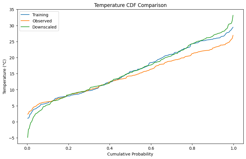
Evaluate Temperature Downscaling
Let’s visualize how well the downscaling corrects the model bias by comparing CDFs.
# Plot overall CDF
fig, ax = plt.subplots(figsize=(10, 6))
plot_cdf(
ax=ax,
Training=X_temp.values.flatten(),
Observed=y_temp.values.flatten(),
Downscaled=temp_downscaled.values.flatten(),
)
ax.set_title('Temperature CDF Comparison')
ax.set_ylabel('Temperature (°C)')
plt.show()
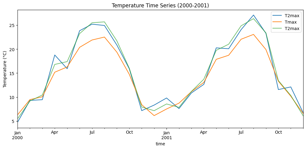
# Plot time series for a sample period
fig, ax = plt.subplots(figsize=(12, 5))
temp_downscaled['2000':'2001'].plot(ax=ax, label='Downscaled')
y_temp['2000':'2001'].plot(ax=ax, label='Observed')
X_temp['2000':'2001'].plot(ax=ax, label='Training', alpha=0.7)
ax.set_title('Temperature Time Series (2000-2001)')
ax.set_ylabel('Temperature (°C)')
ax.legend()
plt.show()
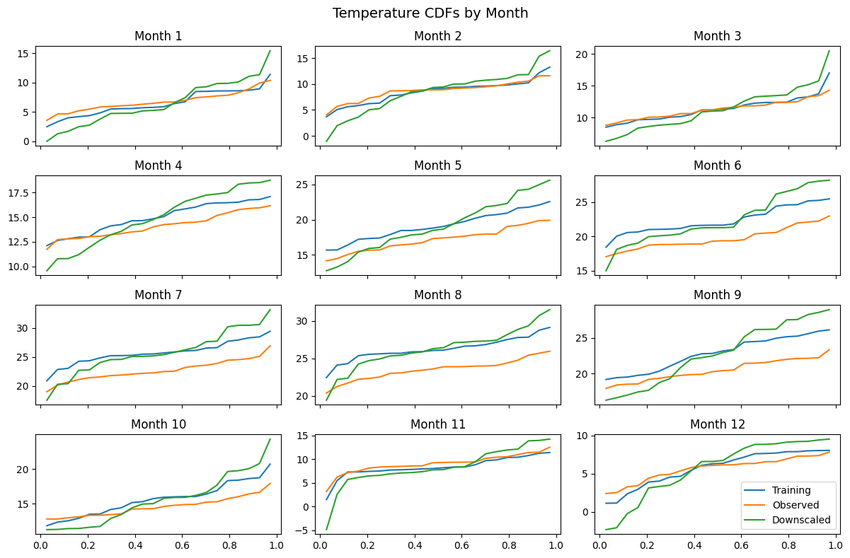
Monthly CDFs for Temperature
Since climate statistics vary by season, let’s examine the CDFs for each month separately.
fig, axes = plot_cdf_by_month(Training=X_temp, Observed=y_temp, Downscaled=temp_downscaled)
fig.suptitle('Temperature CDFs by Month', fontsize=14)
plt.show()
Step 4: Downscale Precipitation with BCSD
Precipitation requires special handling due to its non-Gaussian distribution and the presence of zero values.
Key differences from temperature:
Uses multiplicative (rather than additive) adjustments
Handles zero-precipitation days separately
Uses specialized quantile mapping for non-negative values
# Initialize the BCSD precipitation model
bcsd_pcp = BcsdPrecipitation()

# Fit the model using training data
bcsd_pcp.fit(X_pcp, y_pcp)

# Generate downscaled predictions
# Note: We multiply by X_pcp because the model predicts a scaling factor
pcp_downscaled = bcsd_pcp.predict(X_pcp) * X_pcp

print('Downscaled precipitation (first 5 months):')
display(pcp_downscaled.head())
Downscaled precipitation (first 5 months):
/home/docs/checkouts/readthedocs.org/user_builds/scikit-downscale/envs/latest/lib/python3.13/site-packages/sklearn/utils/validation.py:1406: DataConversionWarning: A column-vector y was passed when a 1d array was expected. Please change the shape of y to (n_samples, ), for example using ravel().
  y = column_or_1d(y, warn=True)
| PREC_TOT | |
|---|---|
| time | |
| 1980-01-01 | 46.673401 |
| 1980-02-01 | 114.921283 |
| 1980-03-01 | 161.957216 |
| 1980-04-01 | 55.210280 |
| 1980-05-01 | 154.597319 |
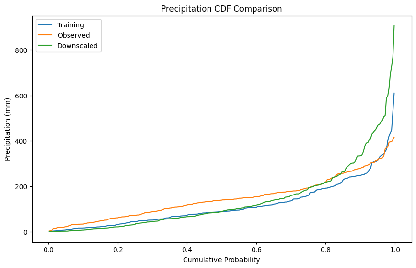
Evaluate Precipitation Downscaling
Let’s compare the statistical properties of our downscaled precipitation with observations.
# Plot overall CDF
fig, ax = plt.subplots(figsize=(10, 6))
plot_cdf(
ax=ax,
Training=X_pcp.values.flatten(),
Observed=y_pcp.values.flatten(),
Downscaled=pcp_downscaled.values.flatten(),
)
ax.set_title('Precipitation CDF Comparison')
ax.set_ylabel('Precipitation (mm)')
plt.show()
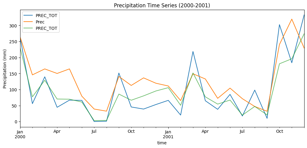
# Plot time series for a sample period
fig, ax = plt.subplots(figsize=(12, 5))
pcp_downscaled['2000':'2001'].plot(ax=ax, label='Downscaled')
y_pcp['2000':'2001'].plot(ax=ax, label='Observed')
X_pcp['2000':'2001'].plot(ax=ax, label='Training', alpha=0.7)
ax.set_title('Precipitation Time Series (2000-2001)')
ax.set_ylabel('Precipitation (mm)')
ax.legend()
plt.show()
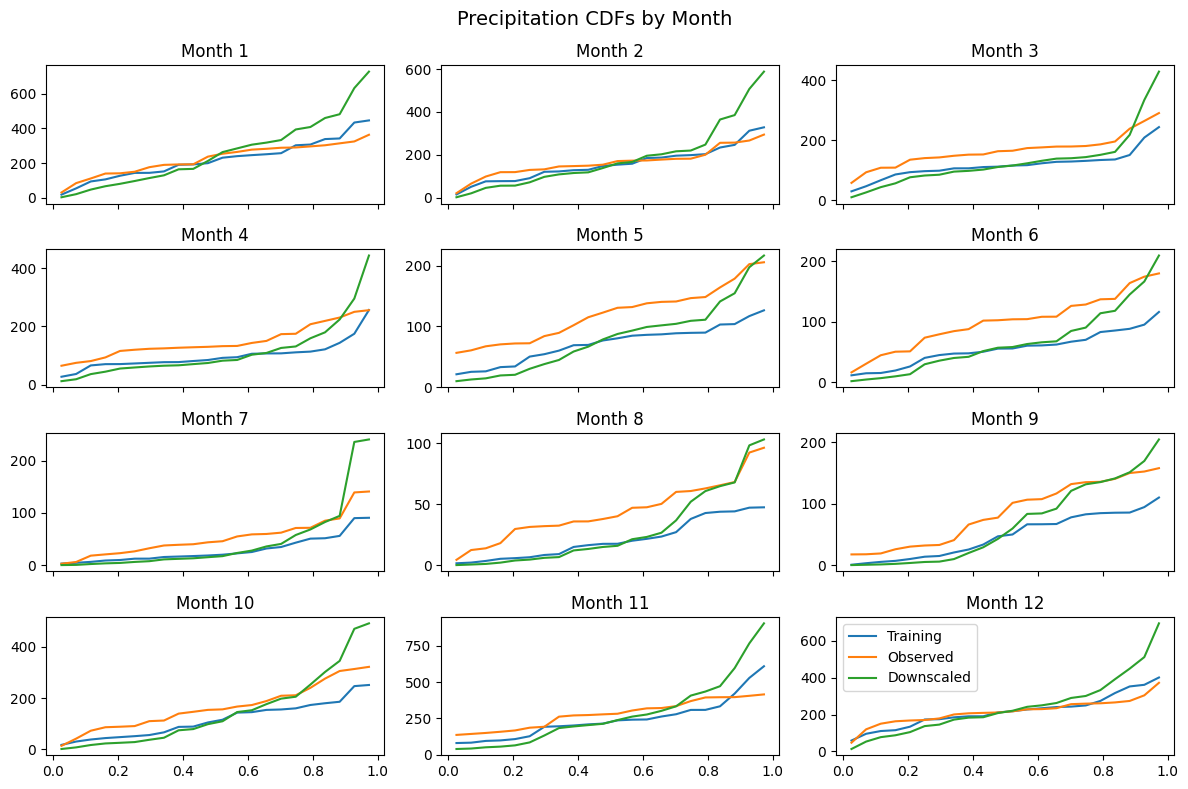
Monthly CDFs for Precipitation
Precipitation patterns often vary significantly by month, so let’s examine monthly CDFs.
fig, axes = plot_cdf_by_month(Training=X_pcp, Observed=y_pcp, Downscaled=pcp_downscaled)
fig.suptitle('Precipitation CDFs by Month', fontsize=14)
plt.show()
Summary
In this tutorial, we demonstrated how to:
✅ Load and prepare climate data from cloud storage
✅ Apply BCSD temperature downscaling using quantile mapping
✅ Apply BCSD precipitation downscaling with special handling for non-negative values
✅ Evaluate results using CDFs and time series plots
Key Takeaways
Temperature: BCSD corrects biases using additive quantile mapping
Precipitation: BCSD uses multiplicative adjustments due to its non-Gaussian nature
Evaluation: CDFs are effective for comparing statistical properties across datasets
Monthly analysis: Examining results by month reveals seasonal performance
Next Steps
Try applying BCSD to multiple spatial points using
PointWiseDownscalerExplore other downscaling methods like GARD or Analog methods
Compare different methods on the same dataset
Apply downscaling to your own climate data
References
Wood, A. W., Leung, L. R., Sridhar, V., & Lettenmaier, D. P. (2004). Hydrological implications of dynamical and statistical approaches to downscaling climate model outputs. Climatic Change, 62(1-3), 189-216.