Getting Started
The Downscaling Workflow
Statistical downscaling typically follows this workflow:
1. Load Data
   ├── Coarse-resolution climate model output (predictor)
   └── High-resolution observations (predictand)

2. Prepare Data
   ├── Align time periods
   ├── Handle missing values
   └── Extract variables of interest

3. Train Model
   └── model.fit(model_data, observations)

4. Generate Predictions
   └── downscaled = model.predict(future_model_data)

5. Evaluate Results
   ├── Compare statistics
   ├── Visualize distributions
   └── Assess temporal patterns
Let’s walk through this workflow step by step!
Setup: Import Libraries
import matplotlib.pyplot as plt
import numpy as np
import pandas as pd
import xarray as xr

# Import downscaling methods
from skdownscale.pointwise_models import BcsdTemperature, PureAnalog, QuantileMapper

# Configure plotting
plt.style.use('seaborn-v0_8-darkgrid')
plt.rcParams['figure.figsize'] = (12, 6)
Step 1: Load Climate Data
We’ll use a small test dataset that includes:
Training data: Climate model output (WRF at 50km resolution)
Target data: Observations (Livneh et al. at 1/16° resolution)
This data is hosted in cloud storage for easy access.
# Load data from cloud storage
data = xr.open_datatree(
    's3://carbonplan/share/scikit-downscale/test-data.zarr',
    engine='zarr',
    chunks={},
    storage_options={'anon': True, 'endpoint_url': 'https://rice1.osn.mghpcc.org'},
)

# Extract datasets for the training period (1980-2001)
training_period = slice('1980', '2001')
training_data = data['training'].to_dataset().sel(time=training_period)
target_data = data['targets'].to_dataset().sel(time=training_period)

print('📊 Training Data (Climate Model Output):')
print('=' * 60)
display(training_data)

print('\n📊 Target Data (Observations):')
print('=' * 60)
display(target_data)
📊 Training Data (Climate Model Output):
============================================================
<xarray.Dataset> Size: 2MB
Dimensions:      (point: 5, time: 8036)
Coordinates:
  * time         (time) datetime64[ns] 64kB 1980-01-01T11:30:00 ... 2001-12-3...
    lat          (point) float32 20B dask.array<chunksize=(5,), meta=np.ndarray>
    lon          (point) float32 20B dask.array<chunksize=(5,), meta=np.ndarray>
Dimensions without coordinates: point
Data variables: (12/15)
    DIV          (point, time) float32 161kB dask.array<chunksize=(3, 8036), meta=np.ndarray>
    PREC_ACC_C   (point, time) float32 161kB dask.array<chunksize=(3, 8036), meta=np.ndarray>
    PREC_ACC_NC  (point, time) float32 161kB dask.array<chunksize=(3, 8036), meta=np.ndarray>
    PREC_TOT     (point, time) float32 161kB dask.array<chunksize=(3, 8036), meta=np.ndarray>
    PSFC         (point, time) float32 161kB dask.array<chunksize=(3, 8036), meta=np.ndarray>
    QVAPOR       (point, time) float32 161kB dask.array<chunksize=(3, 8036), meta=np.ndarray>
    ...           ...
    T2min        (point, time) float32 161kB dask.array<chunksize=(3, 8036), meta=np.ndarray>
    T_MEAN       (point, time) float32 161kB dask.array<chunksize=(3, 8036), meta=np.ndarray>
    T_RANGE      (point, time) float32 161kB dask.array<chunksize=(3, 8036), meta=np.ndarray>
    U            (point, time) float32 161kB dask.array<chunksize=(3, 8036), meta=np.ndarray>
    V            (point, time) float32 161kB dask.array<chunksize=(3, 8036), meta=np.ndarray>
    W            (point, time) float32 161kB dask.array<chunksize=(3, 8036), meta=np.ndarray>
Attributes:
    NCO:                        "4.5.5"
    history:                    Wed Mar  1 13:48:35 2017: ncatted -a calendar...
    history_of_appended_files:  Wed Feb  8 14:15:52 2017: Appended file wrf_d...
nco_openmp_thread_number: 1📊 Target Data (Observations):
============================================================
<xarray.Dataset> Size: 707kB
Dimensions:  (time: 8036, point: 5)
Coordinates:
  * time     (time) datetime64[ns] 64kB 1980-01-01 1980-01-02 ... 2001-12-31
    lat      (point) float64 40B dask.array<chunksize=(5,), meta=np.ndarray>
    lon      (point) float64 40B dask.array<chunksize=(5,), meta=np.ndarray>
Dimensions without coordinates: point
Data variables:
    Prec     (time, point) float32 161kB dask.array<chunksize=(731, 5), meta=np.ndarray>
    Tmax     (time, point) float32 161kB dask.array<chunksize=(731, 5), meta=np.ndarray>
    Tmin     (time, point) float32 161kB dask.array<chunksize=(731, 5), meta=np.ndarray>
    wind     (time, point) float32 161kB dask.array<chunksize=(731, 5), meta=np.ndarray>
Attributes:
    CDI:                       Climate Data Interface version 1.6.4 (http://c...
    CDO:                       Climate Data Operators version 1.6.4 (http://c...
    Conventions:               CF-1.4
    NCO:                       4.4.5
    history:                   Fri Oct 10 17:54:37 2014: cdo ifthenelse /Volu...
nco_openmp_thread_number: 1Understanding the Data Structure
Dimensions:
time(daily data) andpoint(spatial locations)Training variables:
T2max(max temperature in K),PREC_TOT(precipitation)Target variables:
Tmax(observed max temp in °C),Prec(observed precipitation)
Let’s explore one location in detail.
Step 2: Prepare Data for Analysis
We’ll extract data for a single point and prepare it for downscaling.
# Select a single spatial point (point 0)
point_idx = 0

# Extract and convert temperature data
# Model data: Convert from Kelvin to Celsius
model_temp = training_data.isel(point=point_idx).to_dataframe()[['T2max']] - 273.15
model_temp = model_temp.rename(columns={'T2max': 'temperature'})

# Observed data: Already in Celsius
obs_temp = target_data.isel(point=point_idx).to_dataframe()[['Tmax']]
obs_temp = obs_temp.rename(columns={'Tmax': 'temperature'})

# Align the time indexes (remove time component for daily data)
model_temp.index = model_temp.index.normalize()
obs_temp.index = obs_temp.index.normalize()

print('Model Temperature (first 10 days):')
display(model_temp.head(10))

print('\nObserved Temperature (first 10 days):')
display(obs_temp.head(10))
Model Temperature (first 10 days):
| temperature | |
|---|---|
| time | |
| 1980-01-01 | 7.229950 |
| 1980-01-02 | 6.005737 |
| 1980-01-03 | 4.625702 |
| 1980-01-04 | 3.686951 |
| 1980-01-05 | 1.733826 |
| 1980-01-06 | -2.639313 |
| 1980-01-07 | -2.221100 |
| 1980-01-08 | -3.068573 |
| 1980-01-09 | 0.479004 |
| 1980-01-10 | -1.001953 |
Observed Temperature (first 10 days):
| temperature | |
|---|---|
| time | |
| 1980-01-01 | 7.24 |
| 1980-01-02 | 7.16 |
| 1980-01-03 | 6.53 |
| 1980-01-04 | 4.46 |
| 1980-01-05 | 1.78 |
| 1980-01-06 | 1.37 |
| 1980-01-07 | -0.20 |
| 1980-01-08 | -1.54 |
| 1980-01-09 | -2.06 |
| 1980-01-10 | -0.73 |
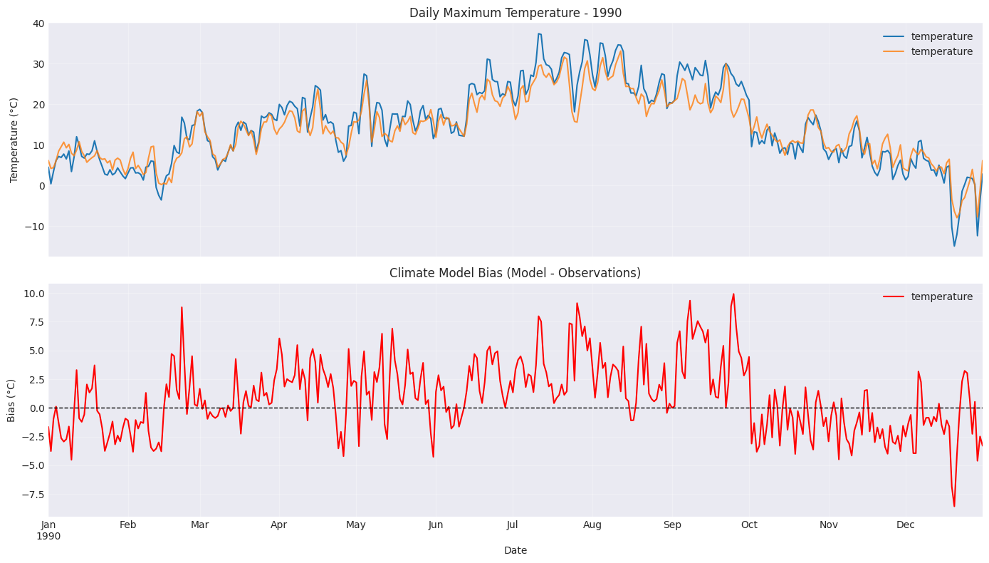
Step 3: Visualize the Problem
Before downscaling, let’s visualize the bias in the climate model.
# Plot one year of data
year_to_plot = '1990'

fig, axes = plt.subplots(2, 1, figsize=(14, 8), sharex=True)

# Time series plot
ax1 = axes[0]
model_temp.loc[year_to_plot].plot(ax=ax1, label='Climate Model', linewidth=1.5)
obs_temp.loc[year_to_plot].plot(ax=ax1, label='Observations', linewidth=1.5, alpha=0.8)
ax1.set_ylabel('Temperature (°C)')
ax1.set_title(f'Daily Maximum Temperature - {year_to_plot}')
ax1.legend()
ax1.grid(True, alpha=0.3)

# Difference plot
ax2 = axes[1]
diff = (model_temp - obs_temp).loc[year_to_plot]
diff.plot(ax=ax2, color='red', label='Model Bias', linewidth=1.5)
ax2.axhline(y=0, color='black', linestyle='--', linewidth=1)
ax2.set_ylabel('Bias (°C)')
ax2.set_xlabel('Date')
ax2.set_title('Climate Model Bias (Model - Observations)')
ax2.legend()
ax2.grid(True, alpha=0.3)

plt.tight_layout()
plt.show()

# Calculate summary statistics
mean_bias = (model_temp - obs_temp).mean().values[0]
rmse = np.sqrt(((model_temp.values - obs_temp.values) ** 2).mean())
print('\n📈 Bias Statistics:')
print(f'   Mean Bias: {mean_bias:.2f}°C')
print(f'   RMSE: {rmse:.2f}°C')
📈 Bias Statistics:
   Mean Bias: 1.14°C
   RMSE: 3.13°C
What We Observe
The climate model shows systematic biases:
The model may consistently over- or under-predict temperatures
Biases may vary by season
Statistical downscaling aims to correct these biases
Step 4: Apply Your First Downscaling Method
Let’s use Quantile Mapping, a popular and effective bias correction method.
How Quantile Mapping Works
Calculate quantiles (percentiles) of model and observed data
Build a mapping function between them
Transform model data to match observed distribution
This is powerful because it corrects biases across the entire distribution, not just the mean.
# Initialize the Quantile Mapper
qm = QuantileMapper()

print('🔧 Training the Quantile Mapper...')
# Fit the model: learn the relationship between model and observations
qm.fit(model_temp, obs_temp)

print('✅ Training complete!')
print('\n🎯 Generating downscaled predictions...')
# Transform: apply the correction to our data
downscaled_array = qm.transform(model_temp)

# Convert back to DataFrame with original index
downscaled_temp = pd.DataFrame(downscaled_array, index=model_temp.index, columns=['temperature'])

print('✅ Downscaling complete!')
print('\nDownscaled temperature (first 10 days):')
display(downscaled_temp.head(10))
🔧 Training the Quantile Mapper...
✅ Training complete!

🎯 Generating downscaled predictions...
✅ Downscaling complete!

Downscaled temperature (first 10 days):
| temperature | |
|---|---|
| time | |
| 1980-01-01 | 7.229950 |
| 1980-01-02 | 6.005737 |
| 1980-01-03 | 4.625702 |
| 1980-01-04 | 3.686951 |
| 1980-01-05 | 1.733826 |
| 1980-01-06 | -2.639313 |
| 1980-01-07 | -2.221100 |
| 1980-01-08 | -3.068573 |
| 1980-01-09 | 0.479004 |
| 1980-01-10 | -1.001953 |
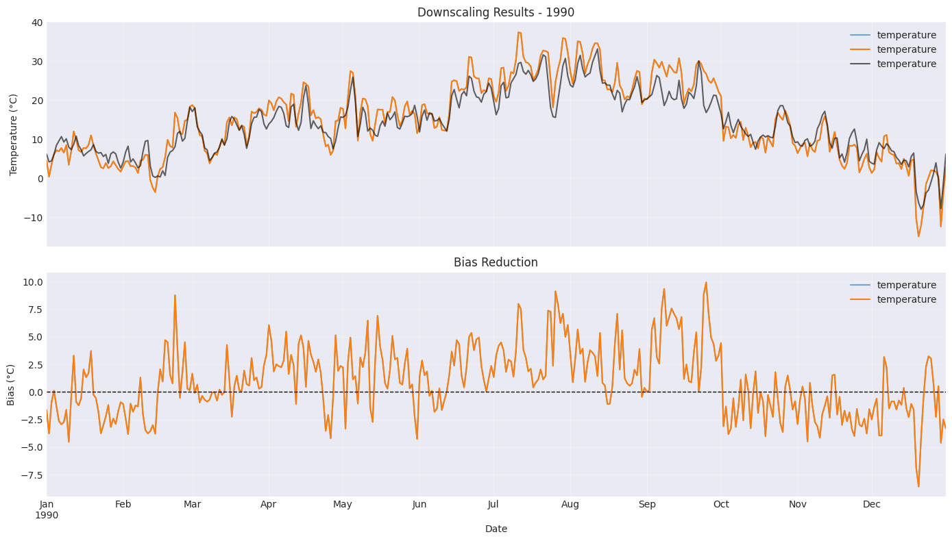
Step 5: Evaluate the Results
Let’s see how well our downscaling performed!
# Plot comparison for the same year
fig, axes = plt.subplots(2, 1, figsize=(14, 8), sharex=True)

# Time series comparison
ax1 = axes[0]
model_temp.loc[year_to_plot].plot(ax=ax1, label='Original Model', linewidth=1.5, alpha=0.6)
downscaled_temp.loc[year_to_plot].plot(ax=ax1, label='Downscaled', linewidth=1.5)
obs_temp.loc[year_to_plot].plot(
    ax=ax1, label='Observations', linewidth=1.5, color='black', alpha=0.6
)
ax1.set_ylabel('Temperature (°C)')
ax1.set_title(f'Downscaling Results - {year_to_plot}')
ax1.legend()
ax1.grid(True, alpha=0.3)

# Bias comparison
ax2 = axes[1]
original_bias = (model_temp - obs_temp).loc[year_to_plot]
downscaled_bias = (downscaled_temp - obs_temp).loc[year_to_plot]

original_bias.plot(ax=ax2, label='Original Bias', linewidth=1.5, alpha=0.6)
downscaled_bias.plot(ax=ax2, label='Downscaled Bias', linewidth=1.5)
ax2.axhline(y=0, color='black', linestyle='--', linewidth=1)
ax2.set_ylabel('Bias (°C)')
ax2.set_xlabel('Date')
ax2.set_title('Bias Reduction')
ax2.legend()
ax2.grid(True, alpha=0.3)

plt.tight_layout()
plt.show()
# Calculate performance metrics
def calculate_metrics(predictions, observations, model_data):
    """Calculate bias correction metrics."""
    # Extract values to ensure proper calculation
    model_vals = model_data.values.flatten()
    obs_vals = observations.values.flatten()
    pred_vals = predictions.values.flatten()

    # Original model metrics
    orig_bias = (model_vals - obs_vals).mean()
    orig_rmse = np.sqrt(((model_vals - obs_vals) ** 2).mean())

    # Downscaled metrics
    ds_bias = (pred_vals - obs_vals).mean()
    ds_rmse = np.sqrt(((pred_vals - obs_vals) ** 2).mean())

    # Correlation
    orig_corr = np.corrcoef(model_vals, obs_vals)[0, 1]
    ds_corr = np.corrcoef(pred_vals, obs_vals)[0, 1]

    return {
        'Original': {'Bias (°C)': orig_bias, 'RMSE (°C)': orig_rmse, 'Correlation': orig_corr},
        'Downscaled': {'Bias (°C)': ds_bias, 'RMSE (°C)': ds_rmse, 'Correlation': ds_corr},
    }


metrics = calculate_metrics(downscaled_temp, obs_temp, model_temp)

# Display as a table
metrics_df = pd.DataFrame(metrics).T
print('\n📊 Performance Comparison:')
print('=' * 60)
display(metrics_df.round(3))

# Calculate improvement
bias_improvement = (
    1 - abs(metrics['Downscaled']['Bias (°C)']) / abs(metrics['Original']['Bias (°C)'])
) * 100
rmse_improvement = (1 - metrics['Downscaled']['RMSE (°C)'] / metrics['Original']['RMSE (°C)']) * 100

print('\n✨ Improvements:')
print(f'   Bias reduced by: {bias_improvement:.1f}%')
print(f'   RMSE reduced by: {rmse_improvement:.1f}%')
📊 Performance Comparison:
============================================================
| Bias (°C) | RMSE (°C) | Correlation | |
|---|---|---|---|
| Original | 1.138 | 3.128 | 0.95 |
| Downscaled | 1.138 | 3.128 | 0.95 |
✨ Improvements:
   Bias reduced by: -0.0%
   RMSE reduced by: 0.0%
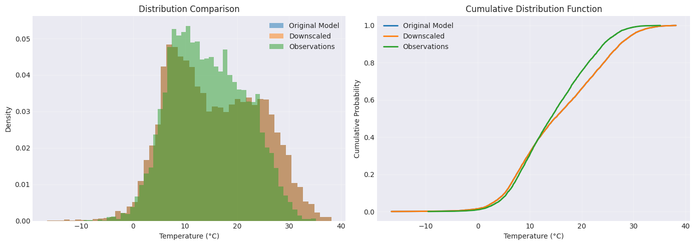
Distribution Comparison
Let’s compare the distributions using histograms and CDFs.
fig, axes = plt.subplots(1, 2, figsize=(14, 5))

# Histogram
ax1 = axes[0]
ax1.hist(model_temp.values, bins=50, alpha=0.5, label='Original Model', density=True)
ax1.hist(downscaled_temp.values, bins=50, alpha=0.5, label='Downscaled', density=True)
ax1.hist(obs_temp.values, bins=50, alpha=0.5, label='Observations', density=True)
ax1.set_xlabel('Temperature (°C)')
ax1.set_ylabel('Density')
ax1.set_title('Distribution Comparison')
ax1.legend()
ax1.grid(True, alpha=0.3)

# Cumulative Distribution Function (CDF)
ax2 = axes[1]
for data, label in [
    (model_temp.values.flatten(), 'Original Model'),
    (downscaled_temp.values.flatten(), 'Downscaled'),
    (obs_temp.values.flatten(), 'Observations'),
]:
    sorted_data = np.sort(data)
    cumulative = np.arange(1, len(sorted_data) + 1) / len(sorted_data)
    ax2.plot(sorted_data, cumulative, label=label, linewidth=2)

ax2.set_xlabel('Temperature (°C)')
ax2.set_ylabel('Cumulative Probability')
ax2.set_title('Cumulative Distribution Function')
ax2.legend()
ax2.grid(True, alpha=0.3)

plt.tight_layout()
plt.show()
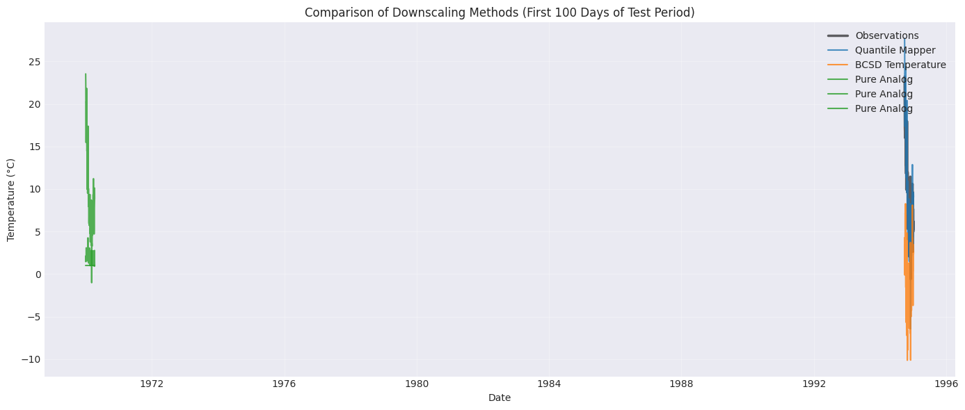
Step 6: Exploring Other Methods
Scikit-downscale includes many downscaling methods. Let’s compare a few!
# Split data for fair comparison
# Use first 2/3 for training, last 1/3 for testing
split_idx = int(len(model_temp) * 0.67)

X_train = model_temp[:split_idx]
y_train = obs_temp[:split_idx]
X_test = model_temp[split_idx:]
y_test = obs_temp[split_idx:]

print(f'Training period: {X_train.index[0]} to {X_train.index[-1]}')
print(f'Testing period: {X_test.index[0]} to {X_test.index[-1]}')

# Compare multiple methods
methods = {
    'Quantile Mapper': QuantileMapper(),
    'BCSD Temperature': BcsdTemperature(),
    'Pure Analog': PureAnalog(kind='mean_analogs', n_analogs=10),
}

results = {}

for name, model in methods.items():
    print(f'\nTraining {name}...')
    model.fit(X_train, y_train)

    # Use transform for QuantileMapper, predict for others
    if hasattr(model, 'predict'):
        predictions = model.predict(X_test)
    else:
        predictions_array = model.transform(X_test)
        # Convert to DataFrame for consistency
        predictions = pd.DataFrame(predictions_array, index=X_test.index, columns=['temperature'])

    results[name] = predictions

    # Calculate RMSE - handle both DataFrame and array
    pred_vals = predictions.values if hasattr(predictions, 'values') else predictions
    obs_vals = y_test.values
    rmse = np.sqrt(((pred_vals - obs_vals) ** 2).mean())
    print(f'  Test RMSE: {rmse:.3f}°C')

print('\n✅ All methods trained!')
Training period: 1980-01-01 00:00:00 to 1994-09-27 00:00:00
Testing period: 1994-09-28 00:00:00 to 2001-12-31 00:00:00

Training Quantile Mapper...
  Test RMSE: 3.390°C

Training BCSD Temperature...
  Test RMSE: 15.788°C

Training Pure Analog...
  Test RMSE: 11.889°C

✅ All methods trained!
/home/docs/checkouts/readthedocs.org/user_builds/scikit-downscale/envs/latest/lib/python3.13/site-packages/sklearn/utils/validation.py:1406: DataConversionWarning: A column-vector y was passed when a 1d array was expected. Please change the shape of y to (n_samples, ), for example using ravel().
  y = column_or_1d(y, warn=True)
# Visual comparison of all methods
fig, ax = plt.subplots(figsize=(14, 6))

# Plot 100 days of test data
plot_slice = slice(0, 100)
test_subset = y_test.iloc[plot_slice]

# Plot observations
ax.plot(test_subset.index, test_subset.values, 'k-', linewidth=2.5, label='Observations', alpha=0.6)

# Plot each method
colors = ['#1f77b4', '#ff7f0e', '#2ca02c']
for (name, predictions), color in zip(results.items(), colors):
    pred_subset = predictions.iloc[plot_slice]
    ax.plot(
        pred_subset.index, pred_subset.values, label=name, linewidth=1.5, alpha=0.8, color=color
    )

ax.set_xlabel('Date')
ax.set_ylabel('Temperature (°C)')
ax.set_title('Comparison of Downscaling Methods (First 100 Days of Test Period)')
ax.legend(loc='upper right')
ax.grid(True, alpha=0.3)
plt.tight_layout()
plt.show()
What’s Next?
Congratulations! You’ve completed your first downscaling workflow. Here are some next steps:
📚 Dive Deeper with Tutorials
BCSD Tutorial: Learn about the Bias Correction Spatial Disaggregation method
Analog Methods Tutorial: Explore pattern-based downscaling approaches
Precipitation Downscaling: Handle the unique challenges of precipitation data
🔧 Advanced Topics
Spatial Downscaling: Apply methods to entire grids using
PointWiseDownscalerCross-validation: Evaluate method performance more rigorously
Custom Methods: Build your own downscaling algorithms
Ensemble Methods: Combine multiple downscaling approaches
📖 Available Methods
Scikit-downscale includes:
Quantile Mapping: Distribution-based bias correction
BCSD: Wood et al.’s Bias Correction Spatial Disaggregation
Analog Methods: Pattern-matching based downscaling
GARD: Generalized Analog Regression Downscaling
Delta Methods: Change-factor approaches
Trend-Aware Methods: Account for non-stationarity